Broadcast Positioning System Deployment in a Single Frequency Network

Nick Hottinger, ONE Media
Liam Power, Edgebeam

Abstract –The Broadcast Positioning System (BPS) encounters complications when utilized in a Single Frequency Network (SFN) environment, as each node of the SFN must transmit the time and location data. In a traditional Multi-Frequency Network (MFN) setup this would not present an issue, but an SFN presents a greater challenge, as the nodes all share the same frequency, and so can potentially interfere with each other. Because BPS is designed to be as receivable as possible, it is difficult to isolate these unique transmissions in the same manner as LDM for local content insertion, and so an alternative approach must be utilized. This paper outlines the background of these issues, describes a solution to resolve them, and provides the results of both real world and lab tests for a multi-node SFN with BPS enabled.

Introduction

Integrated SFN capability is a core component of what makes ATSC 3.0 such a significant leap forward for receivability, as it allows broadcasters to enhance coverage and fill gaps without needing either terrain shielding or a translator license for an additional channel. This enables operators to address the often outlying and urban areas where viewers have some degree of reception, but not enough to successfully retrieve the signal. Simultaneously, BPS is another critical component, due to the nation’s need for a terrestrial GPS backup solution. Going forward, it is likely that both will see increasing usage, and so it is important to ensure this interoperability between the two technologies. This is particularly true for the positioning component of BPS, as SFNs potentially allow for single-channel positioning when enough nodes are receivable, which, as noted in Section 3, is a notable step up over a multi-tuner solution for ease of use.

This paper is divided into the following sections:

• Section 1 – SFN and BPS Overview: A short summary of the two technologies, establishing the context of the deployment scenario.
• Section 2 – Challenges of BPS in an SFN: A description of the real world and lab issues encountered with this usage.
• Section 3 – Solutions to Safely Enable BPS: An overview of the fix discovered to enable viable SFN and BPS implementation, as well as potential future benefits.

Section 1: SFN and BPS Overview

SFN Overview

A single frequency network (SFN) is a mechanism included in the ATSC 3.0 standard that can be used to improve signal coverage of a channel. This is accomplished by deploying additional transmission points beyond the traditional single, high power transmission point used in broadcast deployments. Each site transmits the same signal on the same frequency, improving signal coverage and reach when properly designed by increasing field signal strength through constructive addition and broadcasting into areas that are shadowed from the primary site [7]. 

Broadcast TV stations are licensed to transmit on a 6MHz channel covering an area based on the contour of a transmission antenna at a particular power. Broadcasters will design their transmission system to reach as many people as possible, but there will always be areas that the signal will not cover either due to environmental factors, distance, or a combination of the two. An SFN can help to alleviate this problem, allowing improved signal performance within the designated service contour. The SFN design must still respect the service contour and interference limits of the original channel, so it is not a solution of infinite coverage, but rather a method to improve coverage within the area already licensed by the broadcaster [8]. 

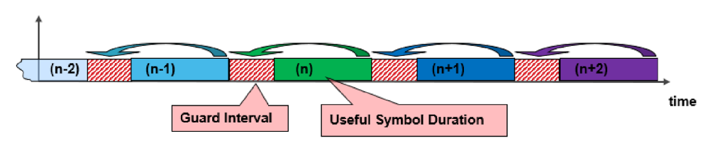
One primary design point for an SFN is the Guard Interval (GI), visually depicted in Figure 1. The Guard Interval is a time buffer that is prepended to each symbol used to prevent inter-symbol interference that occurs from copies of a symbol arriving at different times. This timing difference is naturally present in every transmission with multipath interference where a signal may reflect off of surroundings. The same type of interference is caused by an SFN where propagation distance to a particular site is different from each transmission point. The Guard Interval ensures inter-symbol interference does not become destructive.  However, as with nearly all methods of improved signal reliability, GI adds overhead to the signal, impacting maximum channel capacity. Therefore, the GI should be designed to exceed the maximum propagation delay between SFN transmitters at any given service boundary but should not be needlessly increased as it will cause reduced channel efficiency [4].

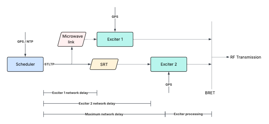
SFNs are designed to transmit at the same time, helping to reduce the potential of misaligned signal arrival at a receiver. The ATSC 3.0 standards include a Bootstrap Reference Time of Emission (BRET) which indicates the precise time that the leading edge of a bootstrap must be emitted from the transmitting antenna [5]. In the evaluated implementation, the exciter generating the ATSC 3.0 signal respects a maximum network delay (MND), a configuration parameter in the scheduler used to define the maximum expected time between STLTP generation and time of signal processing in the exciter, allowing broadcasters to account for any potential network delay for STLTP packet transfer. Respecting the MND has the additional benefit of providing a buffer which allows each transmitter in an SFN to respect the BRET and align transmission. Figure 2 shows a representation of network delay in an SFN. In this example, the primary exciter is connected to the studio via a microwave link, and the secondary site is connected by an IP path utilizing SRT. Despite the difference in delay along the distinct paths, the MND is designed to exceed the longest path. The exciter then processes the signal after the MND, transmitting the signal at the BRET. Along with a properly designed MND, all transmitters should use as close to the same timing source as possible, which is typically accomplished using GPS given the disparate locations of each transmitter.   

BPS Overview

The Broadcast Positioning System (BPS) has been extensively covered in prior papers [1], and forms a core component of the value of a full 3.0 conversion, thanks to the inherent durability and accuracy of the system. One of the primary sources of error in traditional satellite based Global Navigation Satellite Systems (GNSS) is the transit through the atmosphere, which BPS skips entirely. Additionally, BPS has a strong density of sources in much of the United States, thanks to the thousands of towers deployed nationwide, most of which have excellent uptime and redundancy. 

For the purposes of this paper, there are a few key components of BPS that are important to know:

• L1D Timestamp
• Synchronizer/Exciter Infrastructure [2]
• STLTP Bootstrap Reference Emission Time

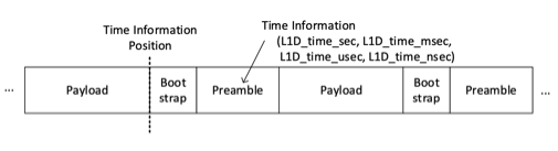
The timestamp is found in the L1D, which is itself part of the ATSC 3.0 preamble. This provides the time of emission for the first symbol of the bootstrap and contains the 32 least significant bits of the number of PTP seconds, plus decimal precision to the nanosecond level. This allows the receiver to determine the current time by noting when the first bootstrap symbol’s first sample was received. This is possible because the exciter is synchronized to an incredibly precise time standard, such as a cesium clock. Figure 3 illustrates the location of the timestamp in the transmission, shown here from left to right over the time domain, as well as the point the time fields are referenced to at the start of the bootstrap.

The cesium clock is used to provide the time in the local network in two ways: it provides a PPS signal to the exciters themselves and the synchronizer for time synchronization, and a 10MHz reference to the synchronizer for frequency synchronization. The synchronizer then uses this reference to analyze the output of the exciter, generating a correction feed which the exciter ingests in order to adjust the emission to more precisely align the timestamp with the sample emission time. This can be seen in Figure 10.

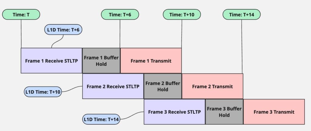
The timestamp itself originates from the STLTP provided by the airchain. As part of the scheduler configuration, the maximum network delay is determined by the operator as defined in the SFN Overview section. The scheduler then sets the timestamp to be a fixed offset into the future from the time of emission of the STLTP from the scheduler. This allows sufficient time for the STLTP to reach every transmitter and be processed, then buffer until the timestamp is reached, at which point the frame begins emission, as seen in Figure 4. With a typical setup, where the exciter is locked to a GPS signal, this is accurate enough for SFN purposes but still has a significant amount of variation due to the limitations of GPS. With BPS, this variation is unacceptable, and so the exciter locks to the feed from the local time standard, allowing it to generate truly accurate time data in combination with the synchronizer.

Section 2: Challenges of BPS in an SFN

LDM, BPS, SFN: Discovering the Problem

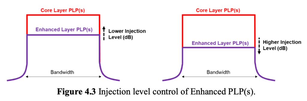
Unfortunately, despite all the benefits of BPS and SFNs, when the two are combined, some trouble can arise. We first noticed some of these issues in the summer of 2025, when we were deploying a new ATSC 3.0 physical configuration to WNUV, a Sinclair-operated station on channel 25 (539 MHz) in Baltimore. This was a layer-division multiplexing (LDM) configuration, as seen in Figure 7, intended to allow mobile and handheld receivers to successfully pull the signal even at speed. In such a configuration, two physical layer pipes (PLPs) are sent simultaneously on the same channel, with one ‘layer’ injected at a lower power than the other, as illustrated in figure 6. This can provide a notable improvement in the bitrate/receivability ratio over a simple time-division multiplexing (TDM) configuration, particularly when the core and enhanced layers have a greater divergence in threshold. In particular, it is commonly used when a broadcaster needs to target both fixed receivers and receivers with less capable antennas or high rates of speed, as the optimal configuration for those situations are on opposite ends of the spectrum. 

	PLP 0	PLP 1	PLP 16
Subframe	0	0	0
Symbols	189	189	189
FFT Size	8K	8K	8K
Guard Interval	512	512	512
Pilot Boost	1	1	1
Reduced Carriers	3	3	3
PLP	0	1	16
Constellation	QPSK	256QAM	QPSK
Code Rate	9/15	7/15	2/15
LDM Layer	Core	Enhanced	Core
Injection Level	N/A	5	N/A
TI Mode	CTI	CTI	CTI
Starting Cell	0	0	1,133,282
Number of Cells	1,133,282	1,133,282	32,400

However, one notable downside of LDM is that it is more complex for receivers to process. Even in an ideal world, this makes it easy to make mistakes when designing a configuration. Unfortunately, there are also a notable number of non-compliant receivers which fail to fully implement the minimums for the ATSC 3.0 physical layer specification around this component. This means that it is essential to test any planned deployment before pushing it to air, as new incompatibilities are often discovered. Thus, when we received a report of issues with BPS reception two weeks after deploying this new configuration, we immediately assumed it was an LDM issue. 

However, one oddity was that the timing data is located in the preamble, which should not have been impacted as part of this change. And indeed, upon loading up Avateq’s BPS receiver, the AVQ 1050, one item stood out: the L1D (L1 Detail – the portion of an ATSC 3.0 preamble that contains the timestamp, amongst other information) [3] Modulation Error Ratio (MER) was extraordinarily low compared to the other components, as seen in Figure 8.

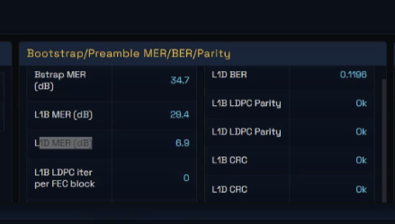
Clearly, something is interfering with the L1D specifically, as if it was simply noise on the channel from a normal interfering transmission, the various components would be expected to see a similar level of drop in MER. The only way to interfere with the L1D specifically, leaving the other components of the signal unaffected, would be to emit another signal precisely timed to the window in which the L1D is transmitted. Ordinarily, this would be almost impossible to occur without a very precise piece of equipment. In this case, however, that piece of equipment not only existed, but had actively been powered on around a month prior. This equipment is, of course, the SFN transmitter located on the Mile One building in Towson, MD. 

In ordinary usage, an SFN results in minimal interference, thanks to the guard interval, which adds a given amount of time between symbols in order to avoid inter-symbol interference (ISI). This is a major factor in making ATSC 3.0 less vulnerable to negative impacts due to multipath. Emissions on the same RF channel from multiple SFN nodes is, in effect, multipath, so the guard interval handles that in the same manner. When deploying an SFN, it is critical to select a guard interval high enough to overcome the delta in the echoes from each node at a given location. This, luckily, is a fairly simple math problem, and one that was done for the SFN in the Baltimore market. Had it not been, receivers would see a substantial drop in reception across the board for each component of the signal, not just the preamble.

Instead, the investigation led to a different error source, namely the same timestamp that the analyzer was having trouble receiving. In this setup, the exciter in the primary transmitter was attached to a synchronizer, while the SFN node’s exciter did not have a synchronizer. In a typical 3.0 system, the preamble timestamp is the same on all transmitters, and is dictated by the maximum network delay [5] from the scheduler to each transmitter. The transmitters make best effort to ensure they’re transmitting on the intended time based on the provided timestamp. However, when BPS is enabled in the current design, the exciter is instead adjusting the timestamp based on the feedback received from the synchronizer, as the synchronizer has a far more precise clock than the exciter. This results in a different timestamp on each exciter, as no exciter emits at precisely the same time down to the nanosecond. This can be seen in Figure 9, where after the first frame, the exciters receive a correction indicating that they’re off by 80 and 30 respectively. They therefore adjust the L1D time to match, resulting in an emission perfectly on time, but at two different times, resulting in the L1D Time field varying between the two, and thus causing this interference.  Note that unlike in the figure, the error in a a true BPS environment is not a constant, and so requires continuously variable correction.

In the WNUV case, where one of the exciters didn’t have a synchronizer at all, the gap is even more pronounced, but as long as there is some difference in the numbers, the symbols will vary. Once different signals are present, the system is now effectively jamming itself. This is only noticeable when the receiver is pulling both the primary and secondary nodes sufficiently well, either due to being near the SFN or having a sufficiently capable receive apparatus. Of course, the monitoring system has an excellent antenna to ensure consistent reception.

	Frame 1		Frame 2
	Exciter 1	Exciter 2	Exciter 1	Exciter 2
L1D Time	500	500	830	780
Actual	580	530	830	780
Correction	+80	+30	+0	+0

To validate this as the cause, we simply disabled the SFN on the Mile One building. This immediately caused the L1D MER to shoot back up, eliminating the BPS reception errors. Turning the SFN back on, then caused the MER to go down to where it had been in Figure 8. With this data in hand, we turned to the lab to narrow down the cause, and to determine if the same results occur even in the ideal deployment when both exciters have synchronizers. 

Lab Test Results

To further investigate the performance of a BPS deployment in an SFN configuration, a lab system was built using a pair of Rohde & Schwartz exciters, Avateq 1050 BPS units acting as synchronizers, and a Safran Rubidium clock as a timing source. Figure 10 depicts the lab setup and signal flow. 

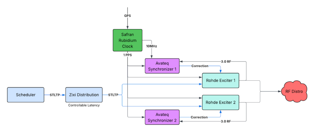
To ensure aligned timing, all devices in the lab configuration utilize the Safran Rubidium clock as both a 1 PPS and NTP source. The Rubidium clock itself uses GPS as a timing source. Each exciter acts as a single transmitter, while the Avateq AVQ 1050 acts as a synchronizer for timing correction on the exciter. The generated signal from each exciter is combined and passed conductively to a set of receivers. A Zixi distribution system was used to establish a controlled STL distribution including configurable distribution latency. The STL signal included a simple set of Audio/Video (A/V) services and a relatively simple physical configuration including a highly robust PLP 16, which is typically used for BPS data transfer. L1D was set to Mode 1, which is typical for ATSC 3.0 channel configurations. Additionally, the setup used a GI of 768, translating to a duration of 111us and an MND of 2000ms was configured. A feature on the exciter called ‘static SFN delay’ was used to control emission timing, allowing the simulation of emission delay resulting in SFN signals arriving at receivers at different times. Using this setup, a variety of tests were conducted, with the most relevant results detailed in Figure 11. 

Test Number	Test Name	Configuration	Test results without BPS correction	Test results with BPS correction
1	Standalone Exciter 1	Exciter 1 On Exciter 2 Off	Power: -62.0 dBm C/N 33.8 dB MER PLP: 32.6 dB MER L1B: 32.6 dB MER L1D: 32.5 dB Service lock on receivers: Success	Power: -61.9 dBm C/N: 33.8 dB MER PLP: 32.6 dB MER L1B: 32.5 dB MER L1D: 32.6 dB Service lock on receivers: Success
2	Standalone Exciter 2	Exciter 1 Off Exciter 2 On	Power: -60.7 dBm C/N: 34.7 dB MER PLP: 33.5 dB MER L1B: 33.4 dB MER L1D: 33.4 dB Service lock on receivers: Success	Power: -60.6 dBm C/N: 34.8 dB MER PLP: 33.5 dB MER L1B: 33.4 dB MER L1D: 33.4 dB Service lock on receivers: Success
3	SFN	Exciter 1 On – SFN Exciter 2 On – SFN	Power: -57.8 dBm C/N: 37.2 dB MER PLP: 26.4 dB MER L1B: 26.1 dB MER L1D: 26.2 dB Service lock on receivers: Success	Power: -57.8 dBm C/N: 37.2 dB MER PLP: 26.5 dB MER L1B: 26.7 dB MER L1D: 1.7 dB Service lock on receivers: Success
4	SFN with network and emission delay	Exciter 1 On – SFN Exciter 2 On – SFN w/ network delay (500ms) and emission delay (50us)	​​Power: -57.9 dBm C/N: 37.2 dB MER PLP: 26.1 dB MER L1B: 26.0 dB MER L1D: 25.9 dB Service lock on receivers: Success	Power: -57.9 dBm C/N: 37.3 dB MER PLP: 26.1 dB MER L1B: 25.9 dB MER L1D: 1.7 dB Service lock on receivers: Success

In each test, the power level, C/N, MER of the PLP, L1B, and L1D, and behavior of service lock was recorded. The measuring device device was an Enensys EdgeProbe and receiver lock was tested with several consumer grade TV and STBs. The recorded metrics should be treated as relative values with the intention of showing general behavior in different configurations. First, each exciter was tested individually with and without BPS timing correction enabled. As detailed in test 1 and 2, signal metrics remain consistent regardless of the presence of BPS timing correction. 

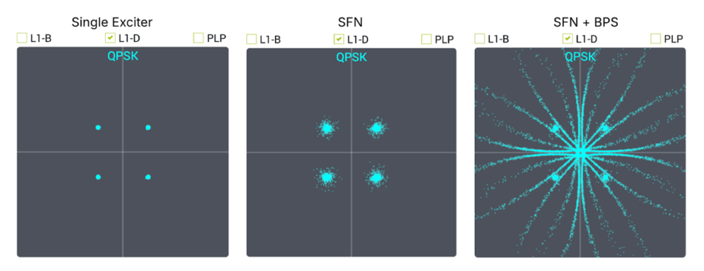
In test 3, SFN is enabled by activating both exciters. This test simulates a nearly ideal SFN setup where there is no STL distribution delay and no emission delay, indicating the receiver will receive both signals nearly simultaneously. Without BPS timing correction enabled, there is a slight improvement to power level and C/N, and a reduction to all MER values. This is the expected and typical behavior of an SFN. In a typical SFN deployment, in areas of signal overlap, power and C/N increase from signal summation, but differential delays between transmitters introduce waveform distortions that reduce MER. When BPS timing correction is enabled, all signal metrics except L1D MER remain consistent. As shown, the L1D MER has a significant reduction. This result clearly shows interference in the L1D and matches the behavior reported in field test results. The impact to L1D MER can be displayed by observing the signal constellation in each configuration. Figure 12 depicts the L1D constellation of the tests included in table X. As shown, the SFN configuration has a small amount of disruption compared to a single exciter, but is still very recognizable as a typical QPSK constellation. Once the timing correction is enabled, significant distortion is observed in the constellation as the L1D symbols are no longer identical. 

To better simulate a real-world setup, two types of delay were added to the SFN configuration in test 4. These delays included an STL distribution delay and an emission delay. The STL distribution delay was set to be 500ms longer to Exciter 2 than exciter 1, simulating a potentially exaggerated version of real world distribution delay difference, but still within the configured MND. The emission delay was set to 50us, ensuring the signals would arrive at the receivers at different times, but still within the Guard Interval. Figure 13 shows the timing difference of the received signals on the receivers. This image includes a depiction of the GI duration and shows two echoes, approximately 50us apart, matching the configured setup. 

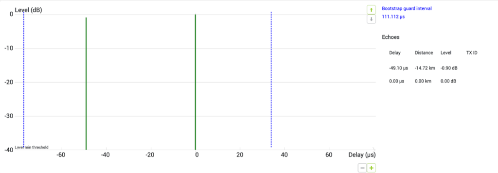
As indicated in the test results, adding STL distribution and emission delays to the system without BPS timing correction had very little impact to the signal metrics. STL distribution delay within the MND should not have an effect on receiver metrics. With longer emission delay, it is possible MER metrics will be reduced, but the signal should remain receivable as long as the signals arrive within the Guard Interval. When BPS timing correction is enabled, the same behavior as recorded in the ideal SFN scenario is found – a significant impact to the L1D MER is observed with no impact to any other signal metric. This indicates the presence of BOS timing correction has caused the interference, while the SFN is behaving exactly as expected within designed parameters. 

One interesting observation in the testing was the lack of an impact to service lock on receivers despite significant degradation to L1D MER performance. Based on the measured L1D MER, this result is not unexpected – when Mode 1 is configured for the L1D, the reception threshold for this portion of the signal is -7.8dB, well below the noise floor. In every test conducted, the L1D did not fall below this threshold. Given the extremely robust nature of L1D in Mode 1, it is possible L1D continues to remain decodable by typical consumer devices and therefore may not result in large disruption to the consumer experience. However, the degradation of L1D presents a major reception risk and will have an impact on BPS receivers which rely on this parameter to be accurate and consistently receivable. 

Section 3: Solutions to Safely Enable BPS

With these results in mind, the question now becomes how to achieve BPS in an SFN environment, without compromising the accuracy of the timestamps. This means that rather than having the timestamp follow the time of emission, the time of emission should instead follow the timestamp, as shown in the table in Figure 14. This ensures that every emitted frame has the same timestamp, dictated by the Studio-to-Transmitter Link Transport Protocol (STLTP) as it is currently in non-BPS deployments. When the preamble is identical, so are the symbols, and so the interference goes away, as the only negative impact is the multipath that the guard interval addresses. 

	Frame 1		Frame 2
	Exciter 1	Exciter 2	Exciter 1	Exciter 2
L1D Time	500	500	750	750
Actual	580	530	750	750
Correction	-80	-30	+0	+0

One key requirement for this, however, is exciter transmission timing accuracy and precision. Currently, even if the exciter timing accuracy is way off target, the synchronizer will be able to compensate for it by adjusting the preamble timestamp to match without negative system impact, assuming the transmission timing precision is fairly narrow. When the variable value becomes the transmit time instead of the preamble time, the exciter now additionally has to be able to accurately transmit the bootstrap at that timestamp. The synchronizer is still able to provide corrections they’re just being applied to a different component of the exciter after this.

Synchronizers in an SFN Environment

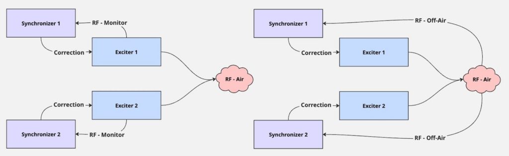
The other critical item for an SFN deployment is the return feed for the synchronizer input. Simply taking an off-air feed will cause the synchronizer to potentially pull multiple nodes of the SFN, throwing off the correction timing, as a) the exciters may be wrong in different directions and degrees and b) the distance will cause differences in the measured vs actual error if it receives from a different site. Instead, the synchronizer should be connected to an isolated monitor feed within the facility before the final transmit antenna, as that will contain only the output of the exciter. An adjustment can be made for the time to travel from this point to the antenna on the tower in order to ensure true accuracy for the time of emission, as this can notably increase the error when operating in the nanosecond and microsecond range. Light travels roughly one thousand feet in a microsecond in air, so a typical tower will add more than a microsecond of delay to the equation. 

SFN for standalone BPS

The positioning function within BPS is derived by a combination of precise timing emission and reception data along with at least three received signals. To avoid the need of a market to build three independent ATSC 3.0 stations with BPS functionality, an important question to consider is whether an SFN can be used to achieve the same functionality. If a single channel BPS was possible, it could represent a significant reduction in receiver complexity and cost by eliminating the need of a multi-tuner solution. 

To allow this functionality, the inherent nature of an SFN to provide an identical signal from each transmission point would need to be slightly modified. There are a few options that could be used to achieve this modification. The first option could be to use Transmitter ID (TxID), an optional parameter that can be used to identify individual transmitters in a network. With each transmitter identified, location data for each transmitter can be included and the precise time of signal arrival from each transmitter could theoretically be determined. TxID is injected at the first Preamble at a controllable injection level. The drawback to this solution is that even at very low injection levels, it impacts the receivability of the Preamble. Given that earlier testing indicated sensitivity to L1D and preamble timing, introducing additional interference may further risk receivability or synchronization performance. Another option could be to precisely offset the transmission of each SFN node. This could theoretically allow a receiver to interpret implied signal reception based purely on relative signal arrival offset. The ATSC 3.0 standards account for this possibility with the parameter tx_time_offset which enables controlled emission in 100ns steps for each transmitter in an SFN [5]. This solution would need to be precisely designed to ensure the offsets do not exceed the GI at any location in the market. 

If technical limitations and considerations can be solved, there are still practical considerations that would impact the feasibility of an SFN acting as a single channel BPS system. SFN are typically designed specifically to improve coverage in underserved areas. As such, there is a high likelihood of areas with no signal overlap. Additionally, perhaps the largest consideration is cost of deployment. In order for this system to work, all areas intended for BPS capability would require SFN overlap of at least 3 signals. While theoretically possible, the scale and cost of deploying sufficient SFN overlap for a single-channel BPS would require careful evaluation before implementation.

Acknowledgements

• Bill Soreth, CPBE, for his excellent feedback and advice on testing configurations.

References

• Mondal, T. Weller, R. D. Matheny, S., “Broadcast Positioning System (BPS) Using ATSC 3.0,” Proceedings of the 2021 NAB Broadcast Engineering and Technology (BEIT) Conference.
• Diamond, P. Mondal, T. Weller, R. Hansen, A. “Delivering Traceable Reference Time for ATSC 3.0-based Broadcast Positioning System (BPS),” Proceedings of the 2023 NAB Broadcast Engineering and Technology (BEIT) Conference.
• ATSC: The Broadcast Standards Association. “ATSC Standard: Physical Layer Protocol,” A/322:2026-01.
• ATSC: The Broadcast Standards Association. “ATSC Recommended Practice: Guidelines for the Physical Layer Protocol,” A/327:2025-07.
• ATSC: The Broadcast Standards Association. “ATSC Standard: Scheduler / Studio to Transmitter Link,” A/324:2025-07
• Rossiter, S. “ATSC (NextGenTV SFN Application,” GatesAir Presentation, October 2022. 
• Schadler, J. Wilhour, R. C., “ATSC 3.0 SFN Network Planning and Antenna Design,” Dielectric LLC, May 2020
• “Effective Date Set for New Rules on TV Distributed Transmission Systems (Single Frequency Networks),” Broadcast Law Blog, 2021.